Lesson 3 Equations and Functions
3.1 Solving Equations
In general we can solve different types of equations to get an exact solution. The solution may be an integer, a fraction, or it may be an expression. Using Maple we can do the same thing using the solve command and obtain an exact solutions for equations and inequalities.
[> solve(2*x-5=7);

[> solve(5*x^2=-6*x);

[> solve(x^2-2*x-1);
[> evalf(%);

[> solve(x^4-4);
[> evalf(%); 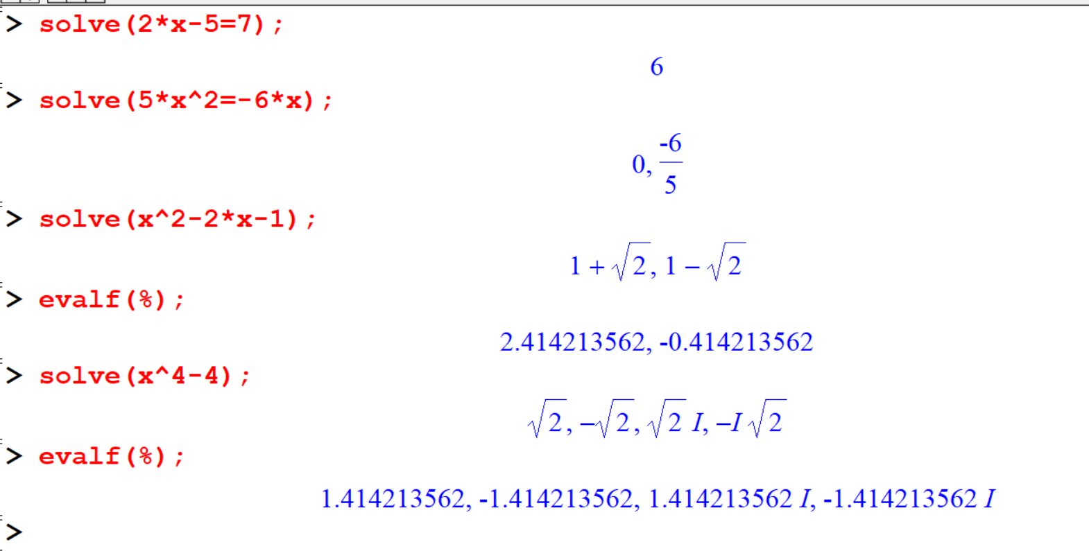
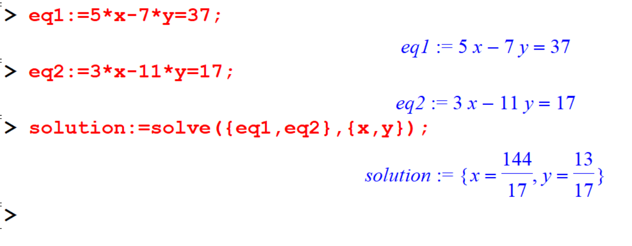
3.2 Equations with multiple unknowns
You can use the solve command to solve equations having several variables. However you have to specify, for which variable that the equation to be solved.
[> solve(a*x^2+b*x+c,x); 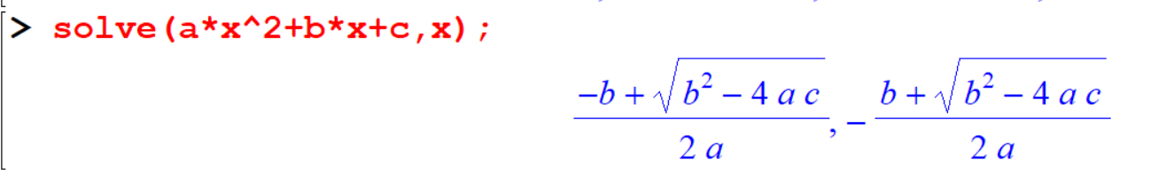
[> eq1:=2*x+3*y-5;
[> solve(eq1,x);
[> solve(eq1,y); 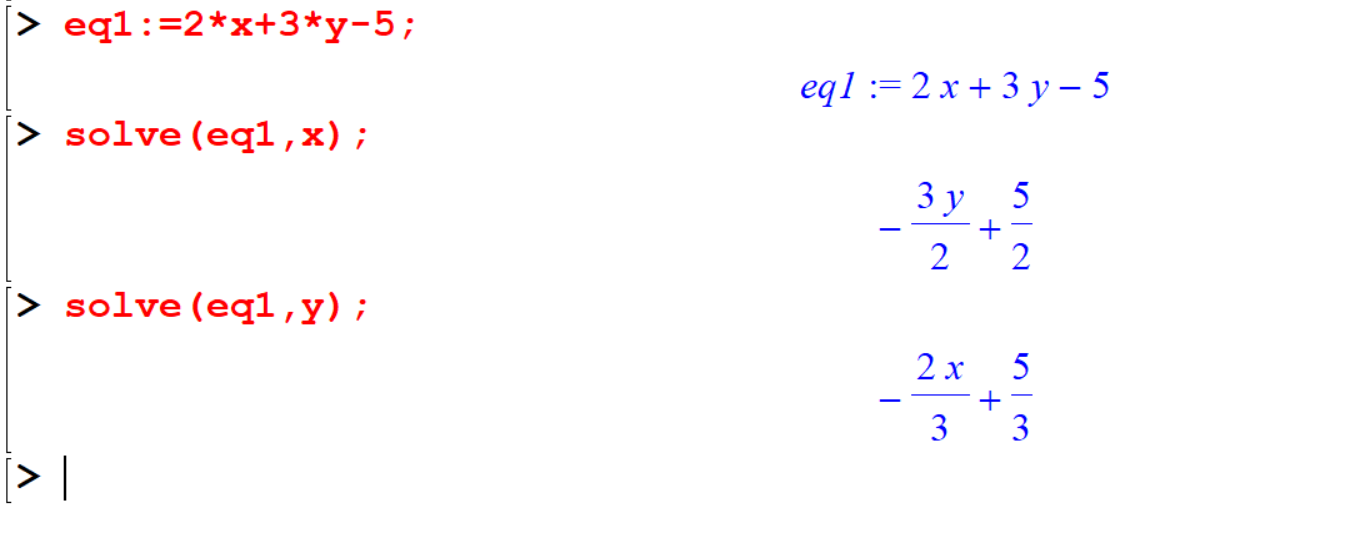
Maple can also solve absolute value equations.
[> restart;
[> eqn1:=abs(3*x+1)=17;
[> solve(eqn1); 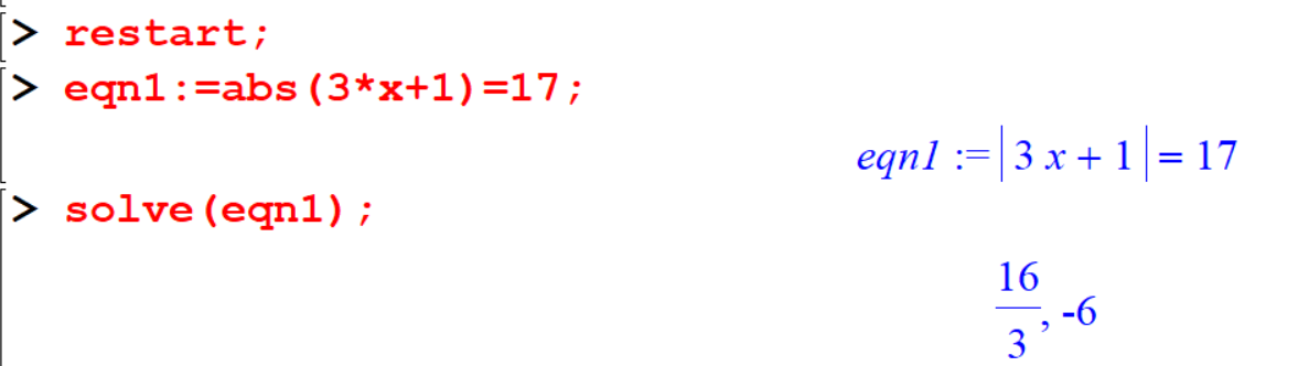
[> eqn2:=abs(41*y-139);
[> solve(eqn2); 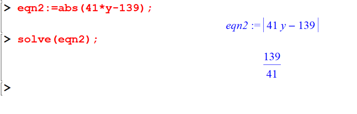
All equations cannot be solved algebraically. It is impossible to find an exact solution.
[> Eq1:=x^5-x+1=0;
[> solve(Eq1);
Using fsolve command we can obtain an approximated numerical value for the answer.
[> fsolve(Eq1);
[> subs(x=-1.167303978,x^5-x+1);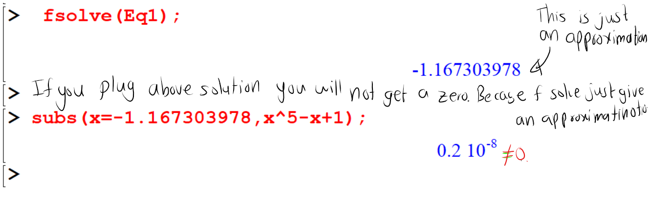
You can see that the solution given is not an exact solution. It’s only an approximation.
[> restart;
[> Eq2:=x^4-4*x=-1;
[> solve(%); 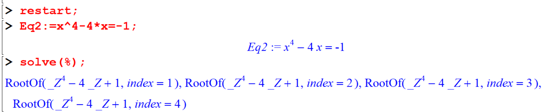 You have to use
 fsolve
[> fsolve(Eq2);
[> subs(x=.2509921575,Eq2);
[> subs(x=1.493358557,Eq2); 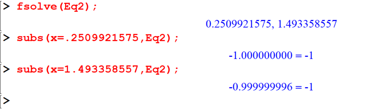
3.3 Functions
Let \(f\) be a function of \(x\). We denote it as \(f(x)\), but in Maple there is a different way to define such functions.
3.3.1 Defining functions
[> restart;
[> f:=x->3*x+1;
[> g:=x->1/(x+2);
[> h:=y->3*y^2+2*y-1;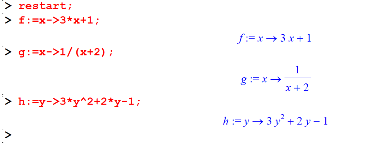 Now you have defined functions, you can evaluate them with numbers, fractions, and irrational numbers.
[> f(-5);
[> g(1000);g(-7/3);
[> g(x);
[> g(t);
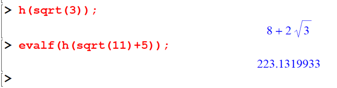
[> h(sqrt(3));
[> evalf(h(sqrt(11)+5)); 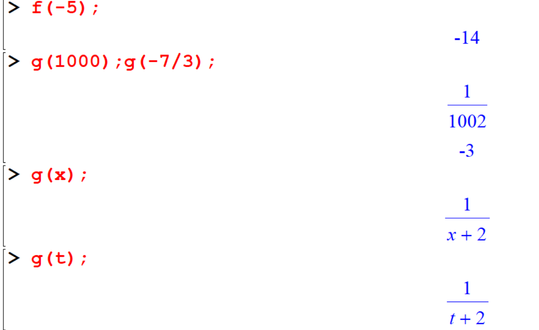
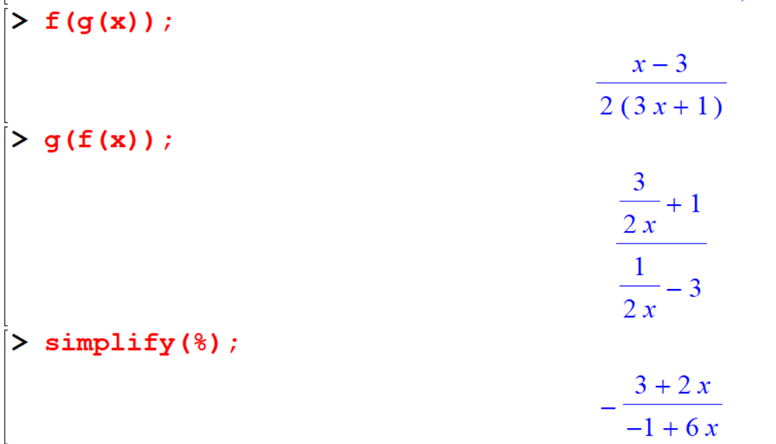
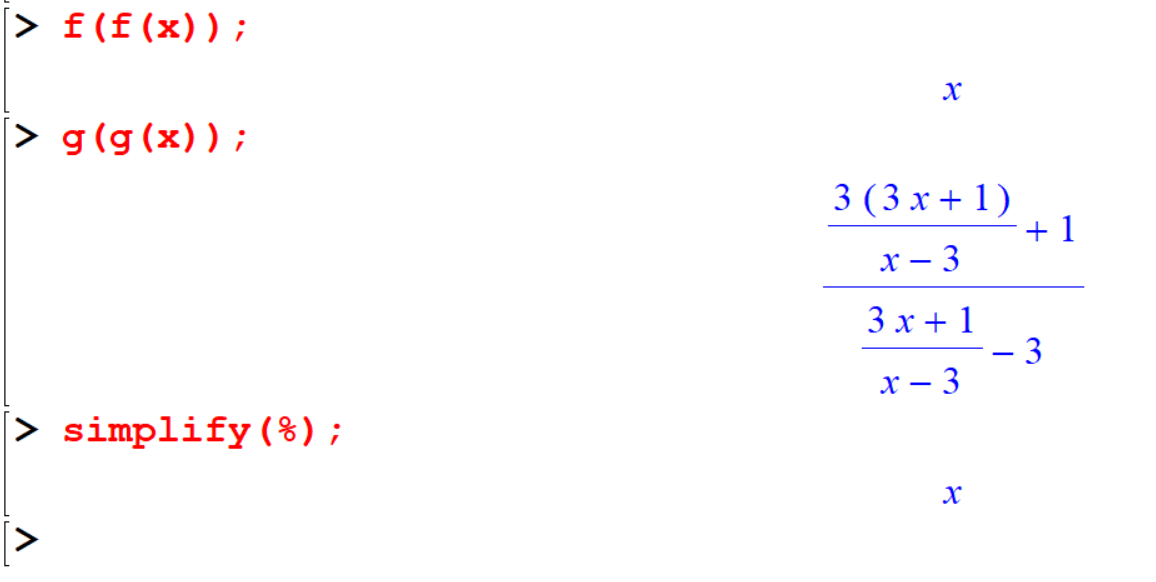
3.3.2 Function Operations and Compositions
You can do +, -, * ,/,\circ between two or more functions.
[> f:=x-> 1/(2*x);
[> g:=x->(3*x+1)/(x-3);
[> f(x)+g(x); #addition of two functions
[> simplify(%);
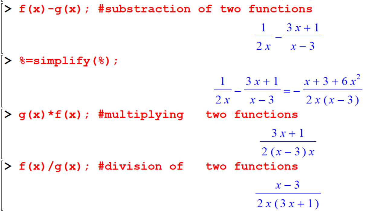
[> f(x)-g(x); #substraction of two functions
[> %=simplify(%);
[> g(x)*f(x); #multiplying two functions
[> f(x)/g(x); #division of two functions
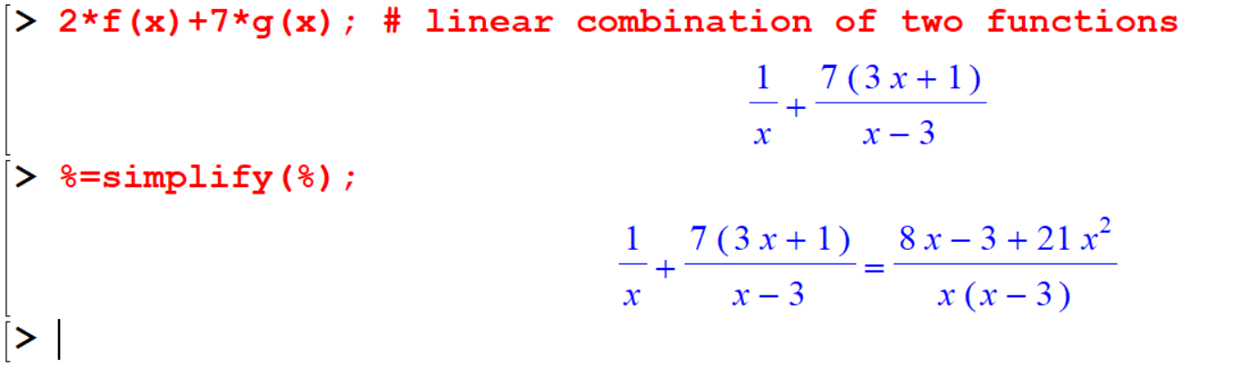
[> 2*f(x)+7*g(x); # linear combination of two functions
[> %=simplify(%); 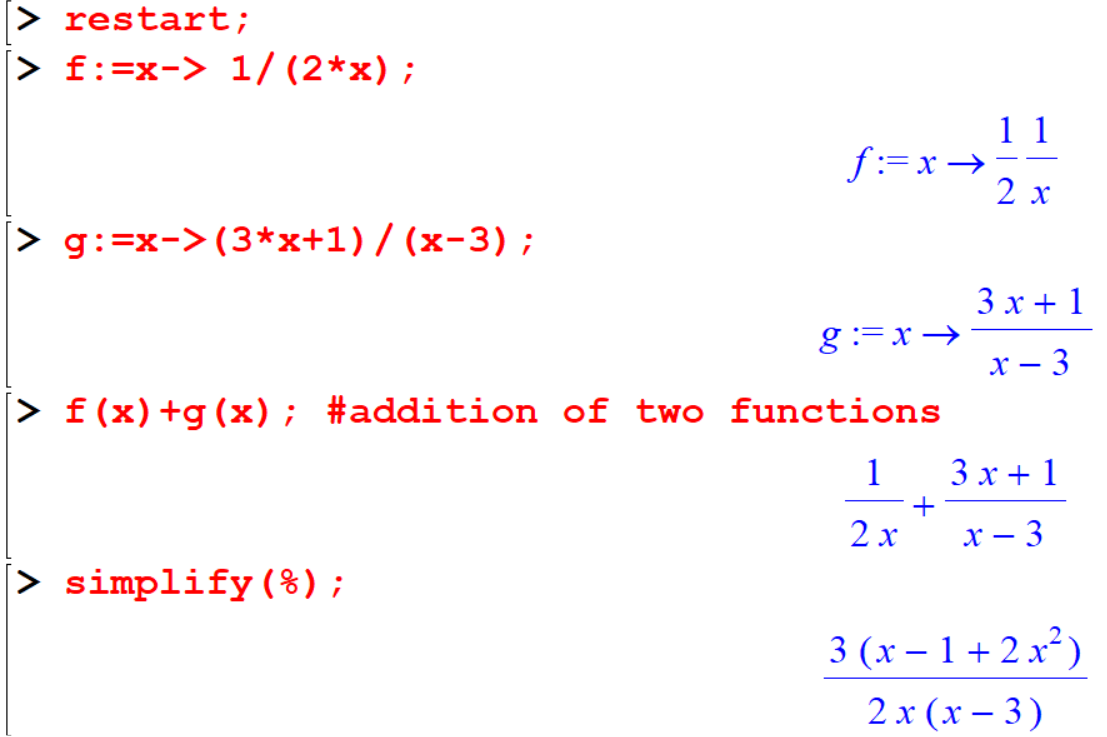
3.4 Trigonometry with Maple
- The Trigonometric functions
\[ \begin{aligned} \sin(x) && \cos(x) && \tan(x) \\ \sec(x) && \csc(x) && \cot(x) \end{aligned} \]
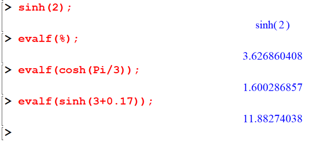
- The Hyperbolic functions
\[ \begin{aligned} \sinh(x) && \cosh(x) && \tanh(x) \\ \text{sech}(x) && \text{csch}(x) && \text{coth}(x) \end{aligned} \]
[> sin(90);
[> evalf(%);
[> sin(Pi/2);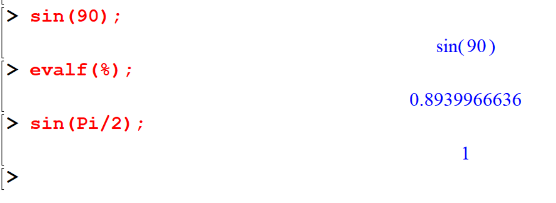
Arguments for all trigonometric and hyperbolic functions must be given in radians. (\(1 \text{radian} = \frac{180}/{\pi} \text{degrees}\))
[> cos(68*Pi/180);
[> evalf(%);
[> cos(Pi/3);
[> evalf(csc(2*Pi/3)); 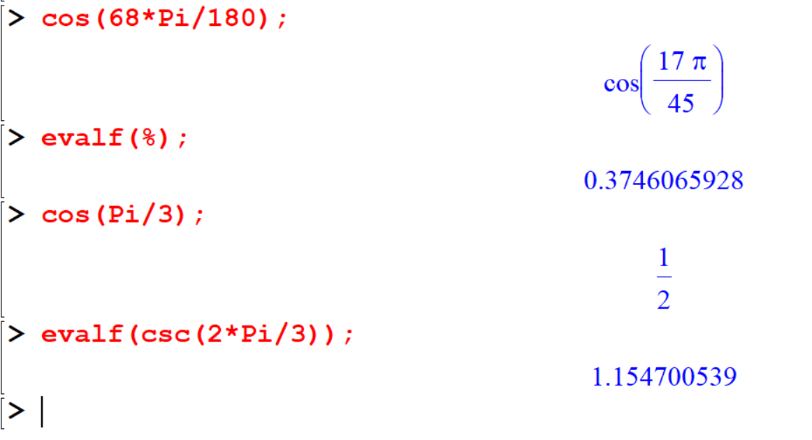
3.4.2 Exponential expansions
The exponential expansions for the trigonometric functions sine and cosine are derived from Euler’s formula:
\[ e^{ix} = \cos(x) + i \sin(x) \]`
By manipulating this formula, we can obtain the expansions:
\[ \begin{align} \sin(x) &= \frac{(e^{ix} - e^{-ix})}{2i}\\ \cos(x) &= \frac{(e^{ix} + e^{-ix})}{2}\\ \tan(x) &= \frac{(e^{ix} - e^{-ix})}{i(e^{ix} + e^{-ix})} \end{align} \] Then, Similarly we can define hyperbolic functions,
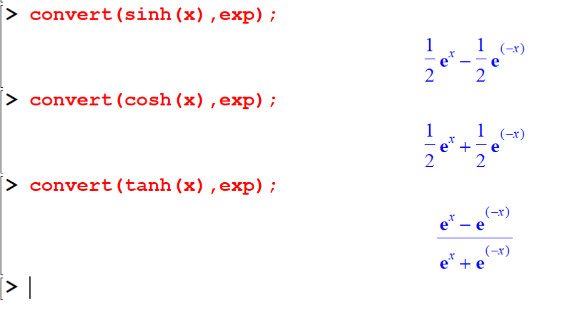
\[ \begin{align} \sinh(x) &= \frac{e^x - e^{-x}}{2}\\ \cosh(x) &= \frac{e^x + e^{-x}}{2} \\ \tanh(x) &= \frac{e^x - e^{-x}}{e^x + e^{-x}} \end{align} \]
You can verify these results with maple
[> convert(sin(x),exp);
[> convert(cos(x),exp);
[> convert(tan(x),exp);
[> convert(sinh(x),exp);
[> convert(cosh(x),exp);
[> convert(tanh(x),exp);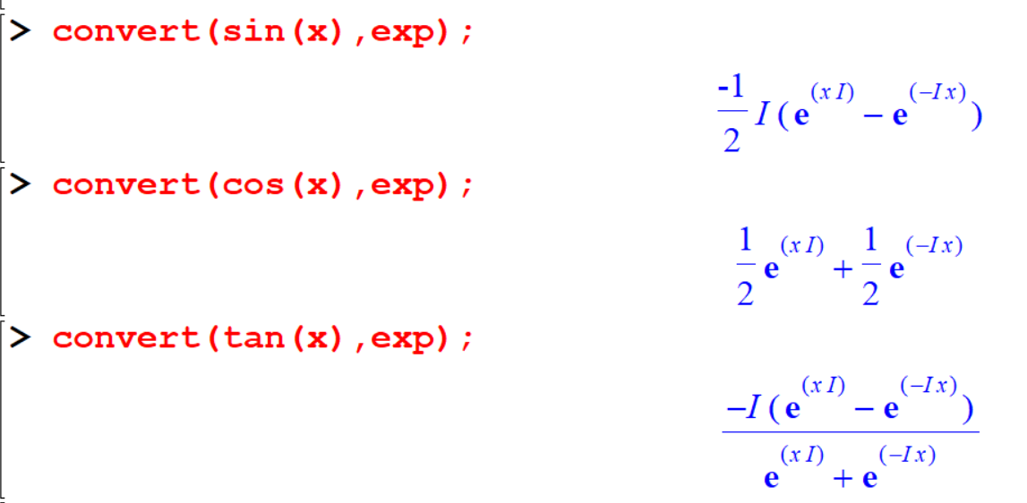
3.4.3 Expanding and simplifying trigonometric functions.
[> expand(sin(2*x));
[> expand(cos(3*x));
[> expand(sin(x+y));
[> simplify(1-(sin(x)^2+cos(x)^2));
[> simplify(1-sin(x)^2+cos(x)^2); 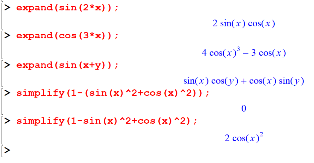
3.4.4 Converting
[> convert(Pi/2,degrees);
[> convert(1,degrees);
[> convert(90*degrees,radians);
[> convert((180/Pi)*degrees,radians);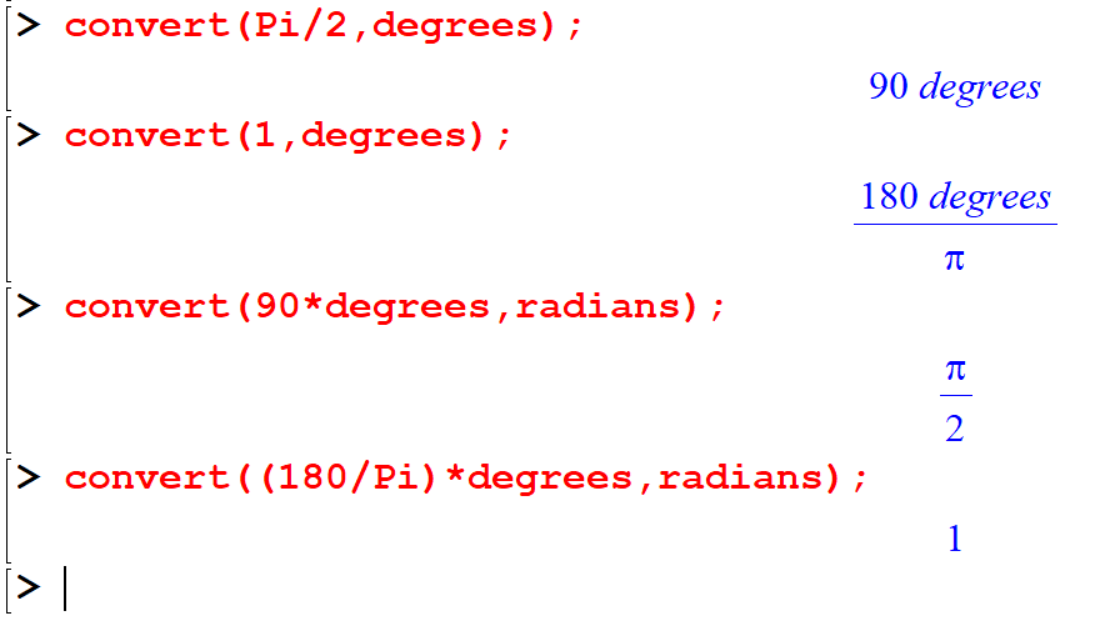
To get an approximate angle, use evalf.
[> evalf(convert(1,degrees));
[> convert(45*degrees,radians);
[> convert(57*degrees,radians);
[> evalf(convert(57*degrees,radians));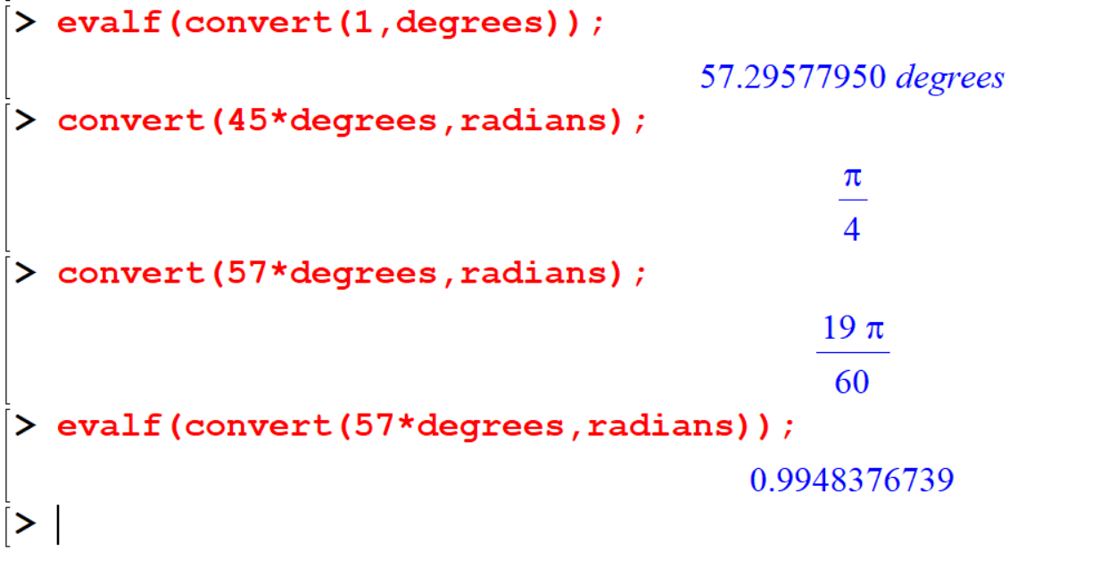
3.5 Inverse trigonometric functions
\[ \begin{aligned} &\arcsin(x) && \arccos(x) && \arctan(x)\\ &\text{arcsec}(x) && \text{arccsc}(x) && \text{arccot}(x)\\ &\text{arcsinh}(x) && \text{arccosh}(x) && \text{arctanh}(x)\\ &\text{arcsech}(x) && \text{arccsch}(x) && \text{arccoth}(x) \end{aligned} \]
The inverse trigonometric and hyperbolic functions are calculated in radians.
[> arcsin(1); 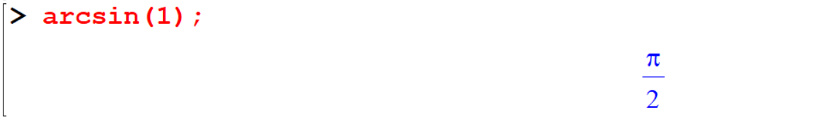 If you need the answer in degrees you have to use
 convert command.
[> arccos(-.05);
[> convert(%,degrees);
[> evalf(%); 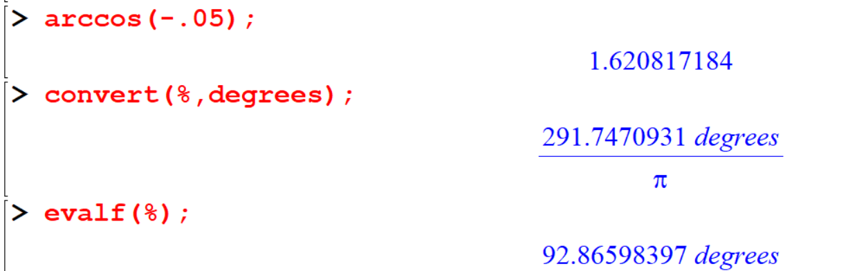
[> sin(arccos(x));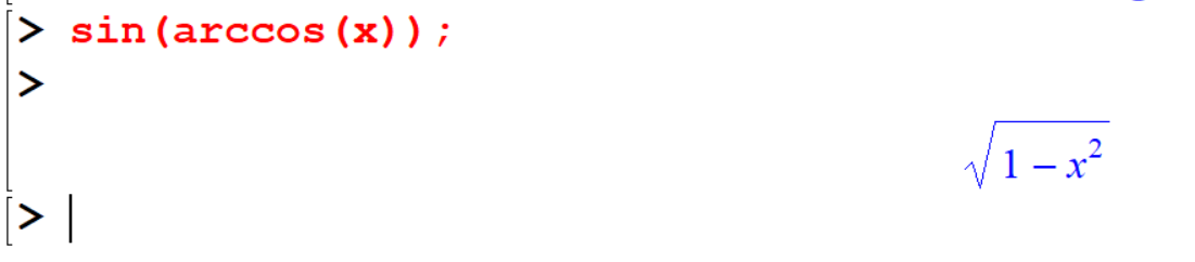
3.6 Exercise
Exercise 3.1 Find the solutions of the following equations to 5 decimal places.
- \(2x^3 + 3x + 1 = 0\)
- \(2x^3 + 3x + \frac{1}{4} = 0\)
- \(x^2 - 13x + 10 = 0\)
- \(-3x + \frac{1}{2}x^2 = 25\)
Exercise 3.2 Find the most accurate real solutions to the following equations.
- \(x^4 - 2x^3 = 7\)
- \(\frac{7}{(x-3)^2} + \frac{5}{(x+5)}\)
Exercise 3.3 Express the following in the form of \(y =mx +c\) using the solve command.
- \(3x + 4y = 2\)
- \(\frac{3y}{5} - 2x + 7 = 0\)
- \(\frac{x}{x-3} + \frac{y}{2x} = -3\)
Use the Maple help to find another way to do the above.
(Hint: You have to isolate y in each equation.)
Exercise 3.4 Consider, \(f(x) = 2x -\frac{x}{3(x+1)}\)
- Define \(f\) as a function: \(f(x) = 2x - \frac{x^3}{x+1}\)
- Evaluate \(f(-\frac{1}{2})\)
- Factor \(f(x)\)
- Simplify \(f(\frac{1}{t-1})\)
Exercise 3.5 Use Maple help to find out how to find logarithms. Then find the value of the following.
- \(\log_{10} 100\)
- \(\ln 100\)
- \(\log_3 10\)
- \(2\log_3 81 + 5\log_8 256\)
Exercise 3.6 Find the value of the following trigonometric expressions for given \(x\).
- \(\sin(\sec(x^2)) + 3x\cos^3(\frac{2x}{7})\), where \(x = 71^\circ\).
- \(\sec^{-1}(\tanh(x+5))\cos(\sec(2x) + \sin(2x))\), where \(x = 43^\circ\).
- \(\left(\cot^{-1}(x) + \sec^{-1}(\frac{x-3}{5})\right)^{\frac{1}{3}}\), where \(x = 71^circ\).