Lesson 7 Differential Equations

7.1 Introduction to differential equations

In this Maple session, we see some of the basic tools for working with differential equations in Maple. First, we need to load the DEtools library: We can find the derivative of a given function by using diff command. - The diff command computes the partial derivative of a given expression with respect to the variables given. - The Diff command returns the unevaluated function. Now consider the following examples.

Example 7.1 Find the derivative of $y=xe^x$ with respect to $x$.

[> with(DEtools):
[> y:=x->x*exp(-x);
[> Diff(y(x),x);
[> diff(y(x),x);
[> Diff(y(x),x)=diff(y(x),x);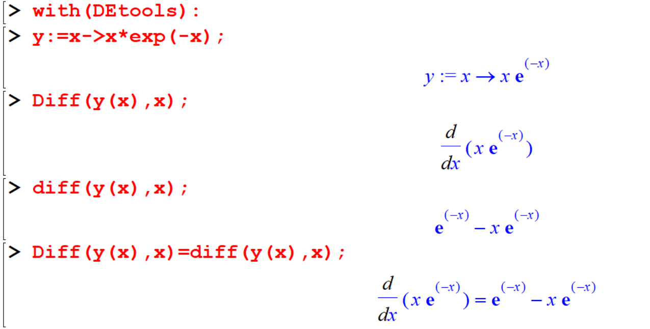

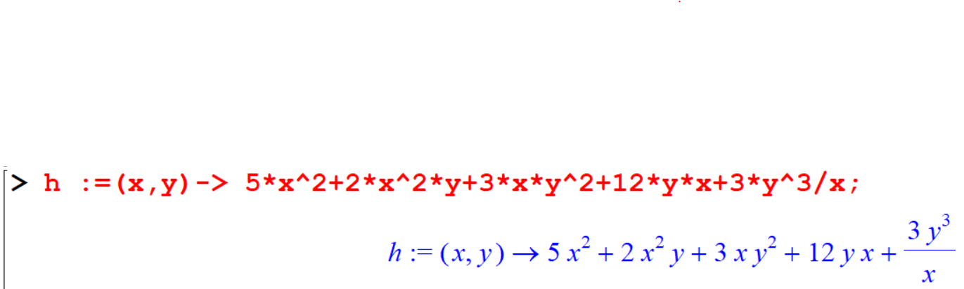
Example 7.2 Consider the follwing function $h$ of two varibels. \[h(x,y)=5x^2 + 2x^2y + 3xy^2 + 12yx + \frac{3y^3}{x}\] Now we are going to differentiate $h$ partially. The next few commands have been done in order to understand the process.

First, we define the function $h$.

[> h :=(x,y)-> 5*x^2+2*x^2*y+3*x*y^2+12*y*x+3*y^3/x;

Then,

[> Diff( h(x,y),x);
[> diff( h(x,y),x);
[> Diff( h(x,y),x)=diff( h(x,y),x);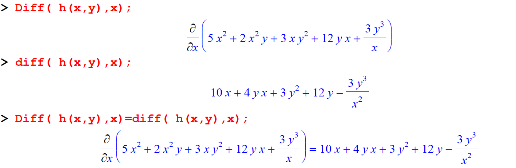

[> Diff(h(x,y),y);
[> diff(h(x,y),y);
[> Diff(h(x,y),y)=diff(h(x,y),y);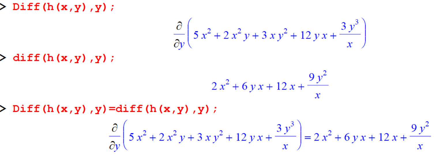

Here we are going to differentiate the function $h$ with respect to $x$ and $y$, using them both in one command. Here the function $h$ should be differentiate first with respect to $x$, and then again with respect to $y$.

[> diff( h(x,y),x,y);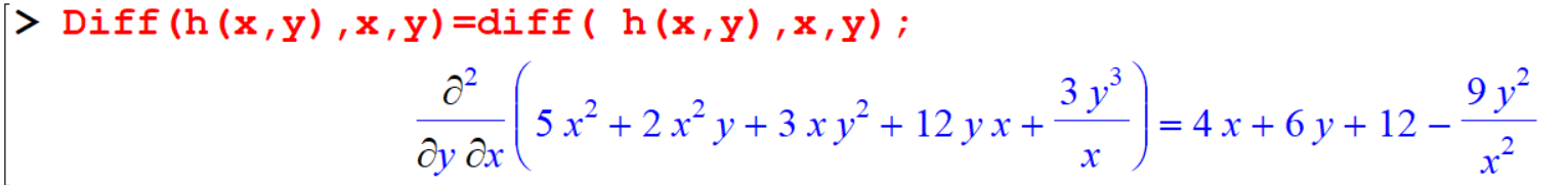

Now, the function h should be differentiate first with respect to $y$, and then again with respect to $x$.

[> diff( h(x,y),y,x);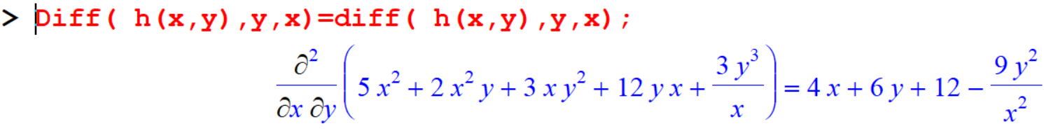

First define the function in Maple. Then you can find the derivative as follows.

Example 7.3 Define the differential equation $y' =y(4-y$

[> diff(y(t),t) = y(t)*(4-y(t));

We cannot drop the ‘$(t)$’ from the dependent variable $y$. Maple treats ‘$y$’ and ‘$y(t)$’ differently, and our equation is for $y(t)$

7.1.1 Exercise

Exercise 7.1 Find the derivatives of the following functions with respect to $x$.

$y = \frac{x^2 + \tan(x^2)}{5x^3 + 9}$
$y = x^{3}\sin(\cos^2(x))$
$y = {(x - 4)^2}{\ln(x)} + \sin(xe^x)$
$y = {3x^3}{\sin^{-1}(x)}$
$y = {\sec^3(x)\cos(2x) + cosec^2(x)}$
$y = x\ln(x) + \cos(2x)e^{5x}$
$y = \frac{e^{2x} + e^{-2x}}{e^{2x} - e^{-2x}}$

7.2 Higher derivatives

Following examples show, how to find higher derivatives of functions.

7.2.1 Method 1

You can find the second derivative by differentiating twice.

[> restart;
[> y:=x->x*exp(-x);
[> Diff(y(x),x,x);
[> d1:=diff(y(x),x);
[> d2:=diff(d1,x);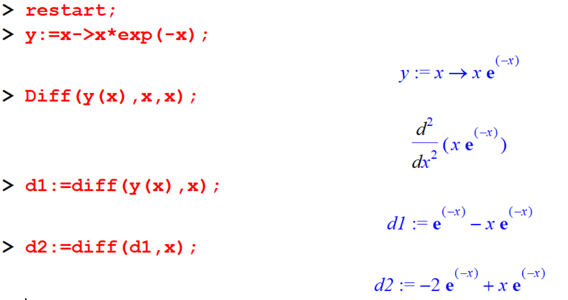

7.2.2 Method 2

You can get the same result by using the following command.

[> d1_2:=diff(y(x),x$2);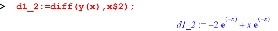

Also you can find higher derivatives by changing $n$. x$n As an example the fifth derivative of the above function as follows.

[> d1_5:=diff(y(x),x$5);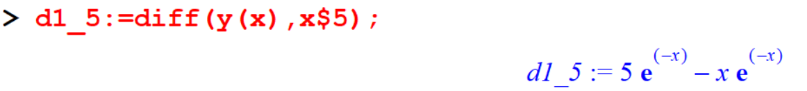

7.2.3 Exercise

Certainly! Let’s express the given expressions in LaTeX and compute their derivatives:

Example 7.4 Let $f(x) = x^2 \sin(kx^3)$.

Compute the 3rd derivative, $f_{xxx}$ of $f(x)$.
Evaluate $f_{xxx}$ at $x = 1$ and $k = 3$.

Example 7.5 Check whether the following functions satisfy the given equations:

If $y = {(1 + \sin(x))^2}$, then $\frac{dy}{dx} - \cos(x) = 2\cos(x)\sin(x) + \cos(x)$.
If $y = x^2 \sin(x)$, then $\frac{8y}{x} - 4\frac{dy}{dx} + x\frac{d^2y}{dx^2} = -(x^2 - 2)\sin(x)$.

7.3 Homogenous Equations

We can check whether a given first order differential equation is homogeneous or not by using the command odeadvisor after loading DEtools package.

Example 7.6 \[\frac{dy}{dx} = \frac{y^2+2xy}{x^2}\]

[> restart;
[> with(DEtools):
[> Eq:=diff(y(x),x)=(y(x)^2+2*x*y(x))/x^2;
[> odeadvisor(Eq);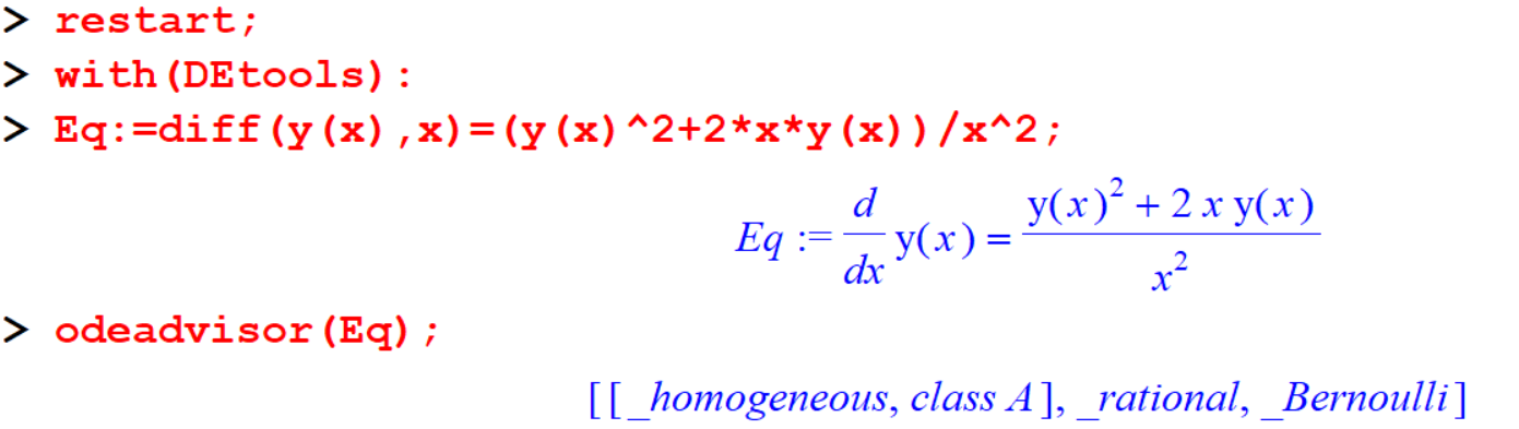

::: {.example #unnamed-chunk-47} \[\frac{dy}{dx} = \frac{xy}{x^2+y^2}\] :::

[> Eq2:=diff(y(x),x)=(x*y(x))/(x^2+y(x)^2);
[> odeadvisor(Eq2);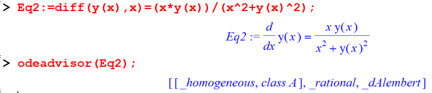

7.4 Solving Differential Equations

The command dsolve is used to solve an ordinary differential equation.

Example 7.7 Solve the differential equation, $\frac{dy}{dx} = -2xy$

[> restart; 
[> with(DEtools):
[> ODE1:=diff(y(x),x)=-2*x*y(x);
[> dsolve(ODE1,y(x));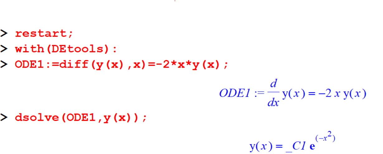

Maple returned the general solution. _C1 denotes, of course, an arbitrary constant. Maple can handle initial value problems also. suppose we have the initial condition $y(0)=2$.

[> dsolve({ODE1,y(0)=2},y(x));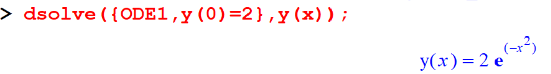

Example 7.8 Example 2: Solve the initial value problem, $\frac{dy}{dx} = 8x^3y^2, \quad y(0) = \frac{1}{2}$

[> dsolve( {diff(y(x), x) = 8*x^3*y(x)^2,y(0)=1/2},y(x));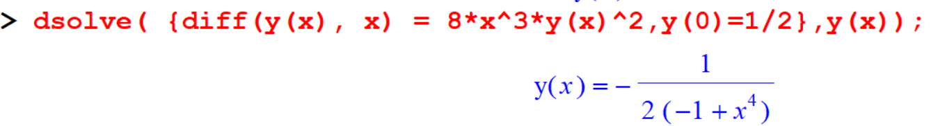

Example 7.9 Solve the initial value problem, $\frac{dy}{dx} + \frac{y}{x} = 1, \quad y(1) = -1$

[> restart;
[> with(DEtools):
[> ODE2:=diff(y(x), x)+y(x) / x =1 ;
[> dsolve({ODE2,y(1)=-1},y(x));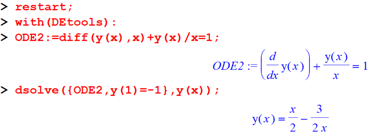

Example 7.10 Solve the initial value problem, $y' = y(4 - y), \quad y(0) = 1$

[> ODE3:=diff(y(t),t)=y(t)*(4-y(t));
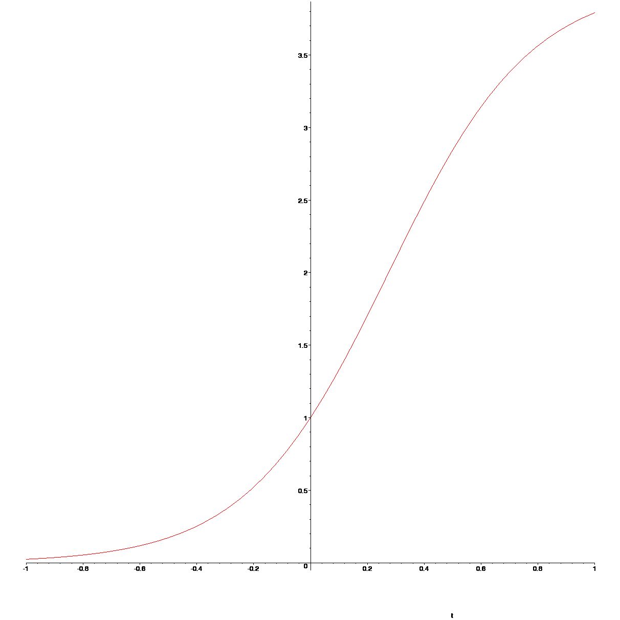
[> sol:=dsolve({ODE3,y(0)=1},y(t));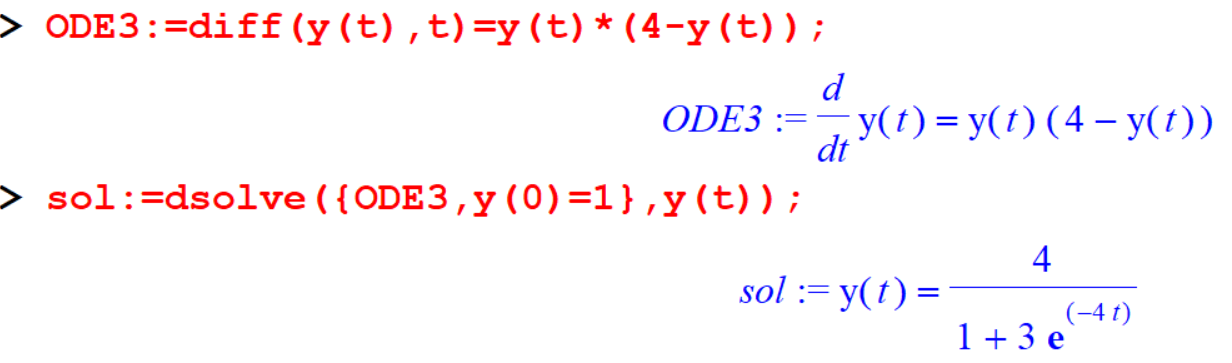

How do we plot this solution?

[> rhsSol:=rhs(sol);
[> plot(rhsSol,t=-1..1);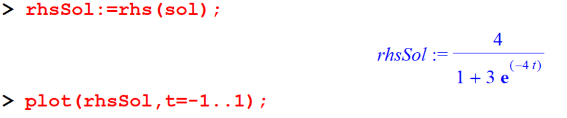

7.5 Direction Fields

A set of short line segment representing the tangent lines can be constructed for a large number of points. This collection of line segment is known as the direction fields of the differential equations.

In Maple you can use the DEplot command, but make sure to load the DEtools package.

DEplot(deqns, vars, xrange, options)

deqns - list or set of first order ordinary differential equations, or a single differential equation of any order
vars - dependent variable, or list or set of dependent variables
xrange - range of the independent variable

Example 7.11 Let see how to graph the direction fields associated with the equation, \[y' = y(4 − y), y(0) = 1\]

[> restart;
[> with(DEtools):
[> ODE3:=diff(y(t),t)=y(t)*(4-y(t));
[> dsolve({ODE3,y(0)=1},y(t));
[> DEplot(ODE3,y(t),t=-1..1,y=-1..5);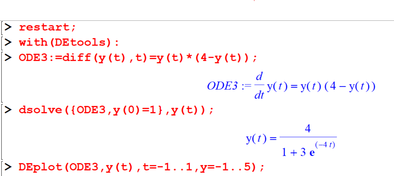

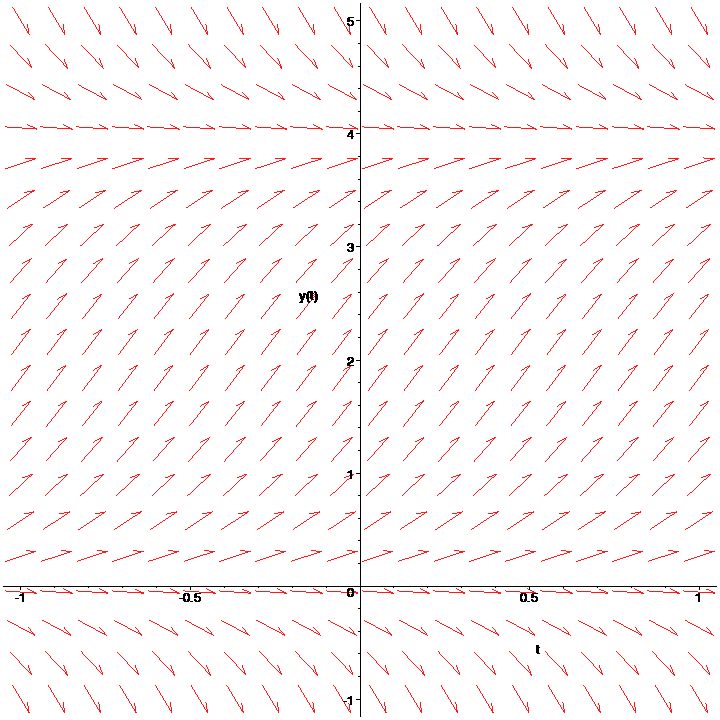
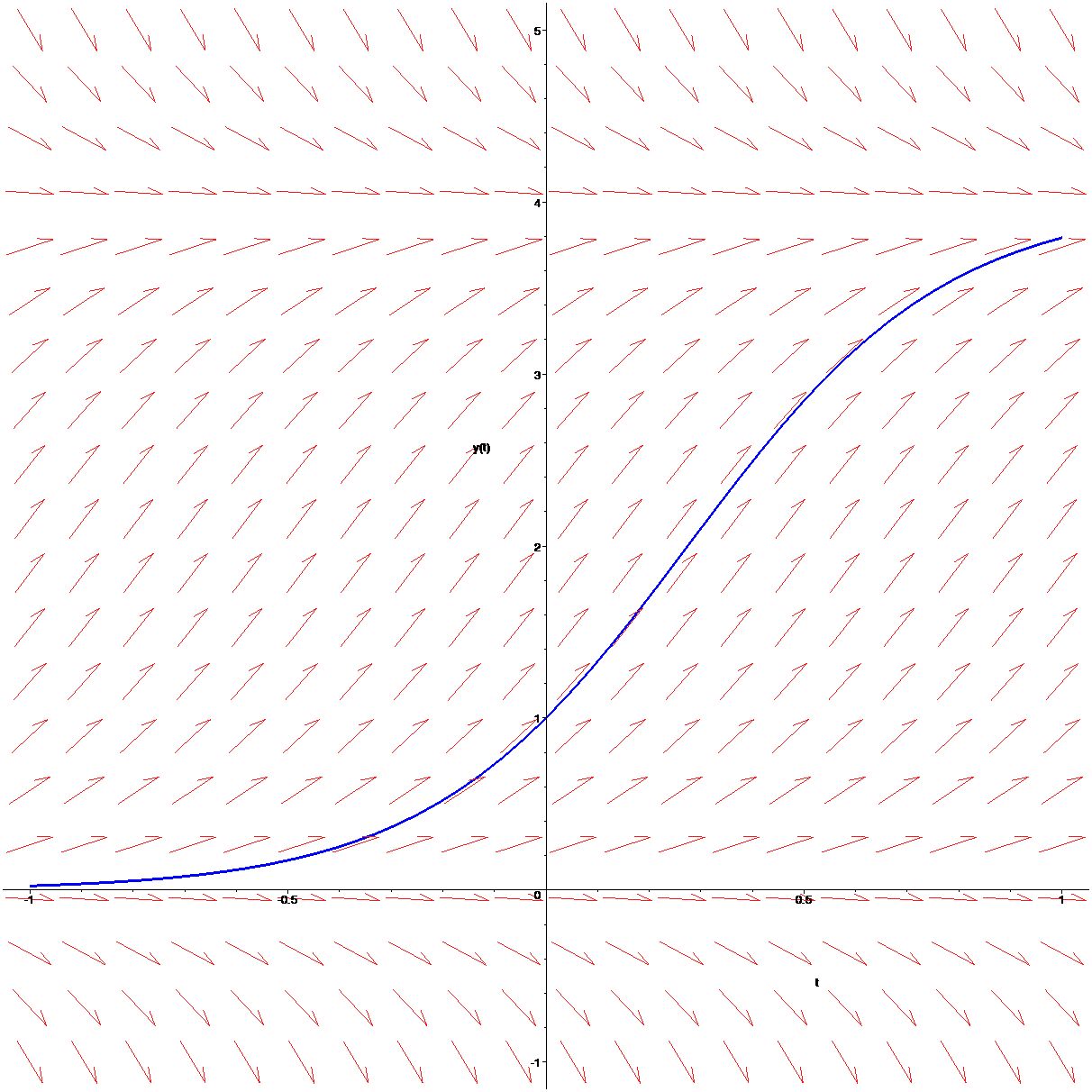
Let’s add a solution curve to this plot. To do this, we must specify an initial condition. Let’s try $y(0)=1$. To specify initial conditions in DEplot, you put them in a list, contained in square brackets,

[> DEplot(ODE3,y(t),t=-1..1,[[y(0)=1]],y=-1..5,linecolor=blue);

You can try out with several initial values as follows:

[> DEplot(ODE3,y(t),t=-1..1,[[y(0)=1],[y(0)=0],[y(0)=1],[y(0)=5]],y=-
1..5,linecolor=[blue,green,black,brown]);

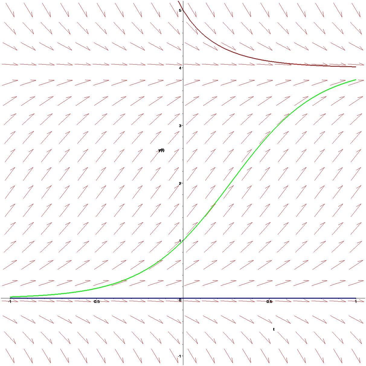
Observe how the arrows drawn in the direction field are tangent to the solution curves.

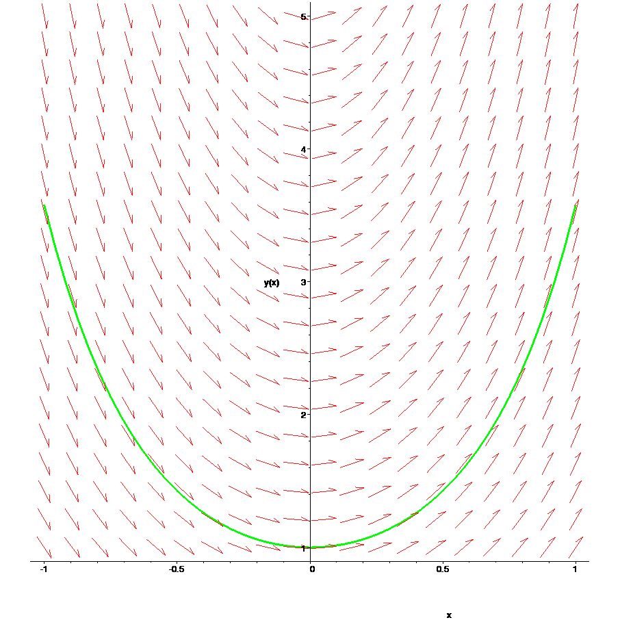
[> Eqn1:=diff(y(x),x)=x+2*x*y(x);
[> DEplot(Eqn1,y(x),x=1..1,[[y(0)=1/2],[y(0)=1]],y(x)=1..5,linecolor=[blue,green]);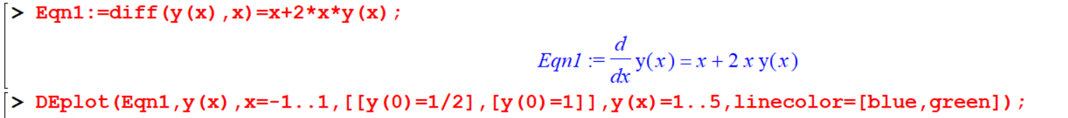

7.6 Exercise

Exercise 7.2 Consider the ODE: $\frac{dy}{dx} = y - x^3$

Find the general solution to the equation.
Plot the direction fields corresponding to the equation for $x$ and $y$ between -2 and 2.
Solve the initial value problems.

$\frac{dy}{dx} = y - x^3$, with $y(0) = {1}$
$\frac{dy}{dx} = y - x^3$, with $y(0) = \frac{1}{2}$

Plot the solution curves and the direction fields in the same graph.

Exercise 7.3

Plot the direction fields for the following equations and state the stability:

$\frac{dy}{dx} = y - 5$
$\frac{dy}{dx} = y(1 - y)$
$\frac{dy}{dx} = y^2(y - 3)$
$\frac{dy}{dx} = y^2 - 5y + 6$
$\frac{dy}{dx} = (y - 3)^2$