Chapter 7 Quantum Computing with Qiskit

Qiskit is an open-source SDK for working with quantum computers at the level of extended quantum circuits, operators, and primitives.
You can find more details in the following PDF file:

Installing Qiskit and Required Packages
Install Qiskit with Visualization Capabilities
# Uncomment and run the following line to install Qiskit with visualization capabilities
# !pip install qiskit[visualization]
Check Qiskit Version
Install Additional Required Packages
# Uncomment the following lines to install other required packages

# %pip install qiskit_aer
# %pip install qiskit_ibm_runtime
# %pip install matplotlib
# %pip install qiskit-transpiler-service
Setting Up the IBM Quantum Environment
Create an account on IBM Quantum and retrieve your API token.

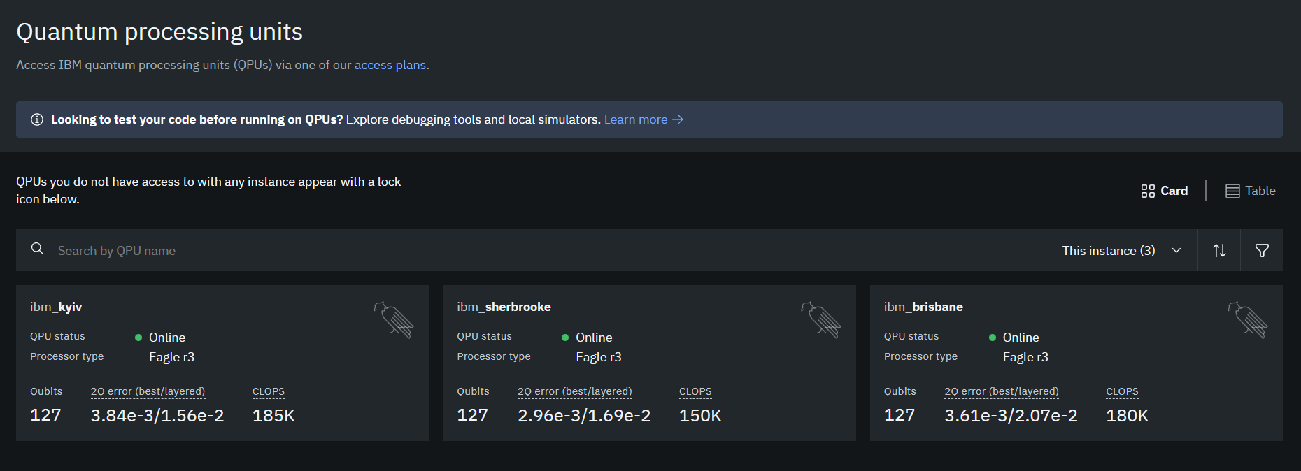
Configuring the Environment
from qiskit_ibm_runtime import QiskitRuntimeService
# Initialize the service with your IBM Quantum token
#service = QiskitRuntimeService(
# channel="ibm_quantum",
# token="YourActualTokenHere" # Replace with your actual token
#)
service = QiskitRuntimeService(channel="ibm_quantum",token = "33")
# Access a specific backend
backend = service.backend(name='ibm_brisbane')
print(f"Backend name: {backend.name}")
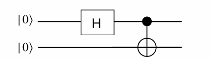
print(f"Number of qubits: {backend.num_qubits}")Let’s try to make the follwing circuits in qiskit.
Example 7.1 .
#Importing QuantumCircuit from qiskit

from qiskit import QuantumCircuit
# Setting the number of qubits

qc=QuantumCircuit(2)
# Importing necessary packages to simulate results

# Designing the circuit by adding Gates and Measurements

qc.h(0)
qc.cx(0,1)
qc.measure_all()

qc.draw(output='mpl')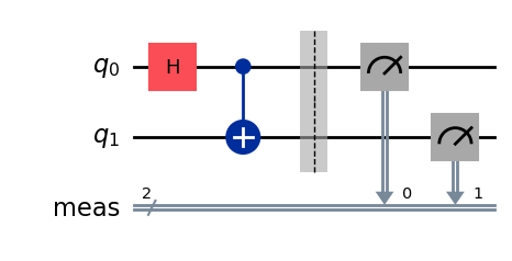
from qiskit import transpile
from qiskit_aer import AerSimulator

backend = AerSimulator()
transpiled_qc = transpile(qc, backend)
job = backend.run(transpiled_qc, shots=100)    # Shots: Numbers of times the algorithm is run and measured
counts = job.result().get_counts()
print(counts)

# Plotting the results from the simulations

from qiskit.visualization import plot_histogram
plot_histogram(counts)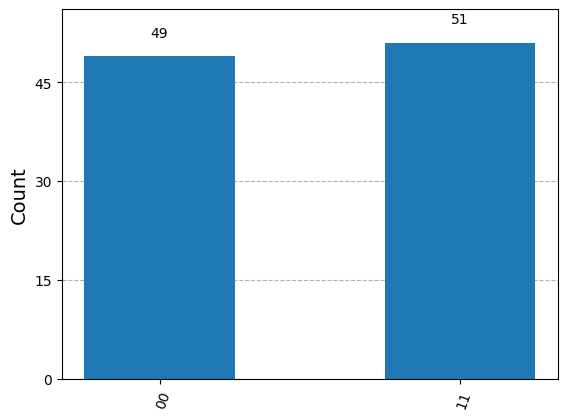
We can verify this result by 3.3.
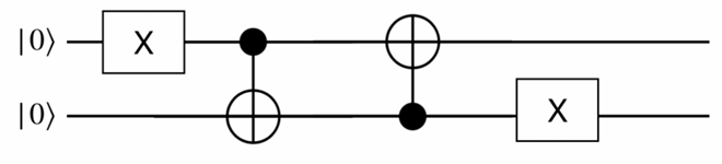
Example 7.2 .
qc2=QuantumCircuit(2)
qc2.x(0)
qc2.cx(0,1)
qc2.cx(1,0)
qc2.x(1)
qc2.measure_all()
qc2.draw(output='mpl')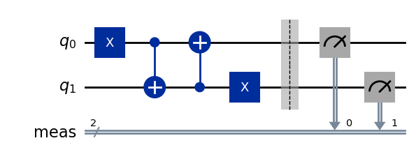
# Importing necessary packages to simulate results

from qiskit import transpile
from qiskit_aer import AerSimulator

backend = AerSimulator()
transpiled_qc2 = transpile(qc2, backend)
job = backend.run(transpiled_qc2, shots=100)    # Shots: Numbers of times the algorithm is run and measured
counts = job.result().get_counts()
print(counts)

from qiskit.visualization import plot_histogram
plot_histogram(counts)
We can verify this result by exercise 3.4
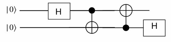
Example 7.3 .
qc3=QuantumCircuit(2)
qc3.h(0)
qc3.cx(0,1)
qc3.cx(1,0)
qc3.h(1)
qc3.measure_all()
qc3.draw(output='mpl')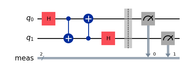
# Importing necessary packages to simulate results

from qiskit import transpile
from qiskit_aer import AerSimulator

backend = AerSimulator()
transpiled_qc3 = transpile(qc3, backend)
job = backend.run(transpiled_qc3, shots=100)    # Shots: Numbers of times the algorithm is run and measured
counts = job.result().get_counts()
print(counts)

from qiskit.visualization import plot_histogram
plot_histogram(counts)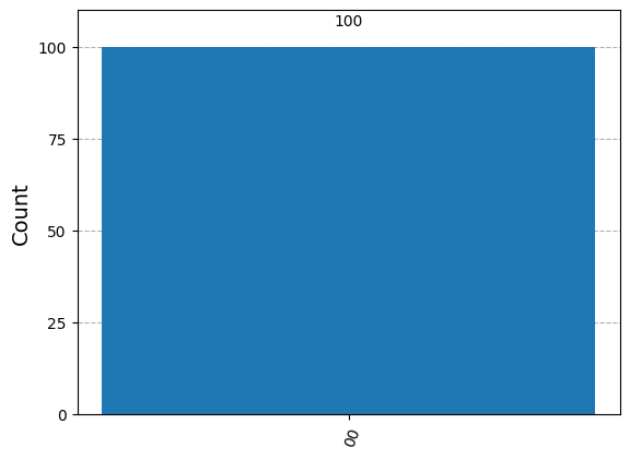
We can verify this result by exercise 3.5
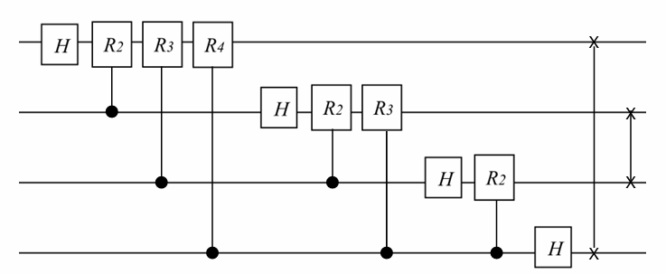
Example 7.4 The circuit implementation of QFT on 4 qubits
from qiskit import QuantumCircuit
import numpy as np

def controlled_rotation(qc, control, target, k):
    """
    Adds a controlled rotation gate R_k to the quantum circuit.

    Parameters:
    qc (QuantumCircuit): The quantum circuit to which the gate is applied.
    control (int): The control qubit index.
    target (int): The target qubit index.
    k (int): The exponent determining the angle of rotation (2π / 2^k).
    """
    # Calculate the rotation angle (2π divided by 2^k)
    angle = 2 * np.pi / (2 ** k)

    # Apply the controlled-phase gate (controlled-R_k)
    qc.cp(angle, control, target)

# Create a 4-qubit quantum circuit
qcF = QuantumCircuit(4)

# Apply a Hadamard gate to qubit 0 to create a superposition
qcF.h(0)  # Hadamard gate on qubit 0

# Apply controlled rotations with qubit 0 as the target
controlled_rotation(qcF, control=1, target=0, k=2)  # Controlled R_2 gate
controlled_rotation(qcF, control=2, target=0, k=3)  # Controlled R_3 gate
controlled_rotation(qcF, control=3, target=0, k=4)  # Controlled R_4 gate
qcF.barrier()  # Add a barrier to separate different sections of the circuit

# Apply a Hadamard gate to qubit 1
qcF.h(1)  # Hadamard gate on qubit 1

# Apply controlled rotations with qubit 1 as the target
controlled_rotation(qcF, control=2, target=1, k=2)  # Controlled R_2 gate
controlled_rotation(qcF, control=3, target=1, k=3)  # Controlled R_3 gate
qcF.barrier()  # Barrier after operations on qubit 1

# Apply a Hadamard gate to qubit 2
qcF.h(2)  # Hadamard gate on qubit 2

# Apply a controlled rotation with qubit 2 as the target
controlled_rotation(qcF, control=3, target=2, k=2)  # Controlled R_2 gate
qcF.barrier()  # Barrier after operations on qubit 2

# Apply a Hadamard gate to qubit 3
qcF.h(3)  # Hadamard gate on qubit 3
qcF.barrier()  # Barrier after operations on qubit 3


# Swap qubits to reverse the order (commonly done in quantum algorithms like QFT)
qcF.swap(0, 3)
qcF.swap(1, 2)

# Measure all qubits
qcF.measure_all()

# Print the quantum circuit
print(qcF)

# Draw the quantum circuit diagram
qcF.draw(output='mpl')Output:
      ┌───┐                            ░                         ░      »
 q_0: ┤ H ├─■────────■────────■────────░─────────────────────────░──────»
      └───┘ │P(π/2)  │        │        ░ ┌───┐                   ░      »
 q_1: ──────■────────┼────────┼────────░─┤ H ├─■────────■────────░──────»
                     │P(π/4)  │        ░ └───┘ │P(π/2)  │        ░ ┌───┐»
 q_2: ───────────────■────────┼────────░───────■────────┼────────░─┤ H ├»
                              │P(π/8)  ░                │P(π/4)  ░ └───┘»
 q_3: ────────────────────────■────────░────────────────■────────░──────»
                                       ░                         ░      »
meas: 4/══════════════════════════════════════════════════════════════════»
                                                                        »
«                  ░       ░        ░ ┌─┐
«   q_0: ──────────░───────░──X─────░─┤M├─────────
«                  ░       ░  │     ░ └╥┘┌─┐
«   q_1: ──────────░───────░──┼──X──░──╫─┤M├──────
«                  ░       ░  │  │  ░  ║ └╥┘┌─┐
«   q_2: ─■────────░───────░──┼──X──░──╫──╫─┤M├───
«         │P(π/2)  ░ ┌───┐ ░  │     ░  ║  ║ └╥┘┌─┐
«   q_3: ─■────────░─┤ H ├─░──X─────░──╫──╫──╫─┤M├
«                  ░ └───┘ ░        ░  ║  ║  ║ └╥┘
«meas: 4/══════════════════════════════╩══╩══╩══╩═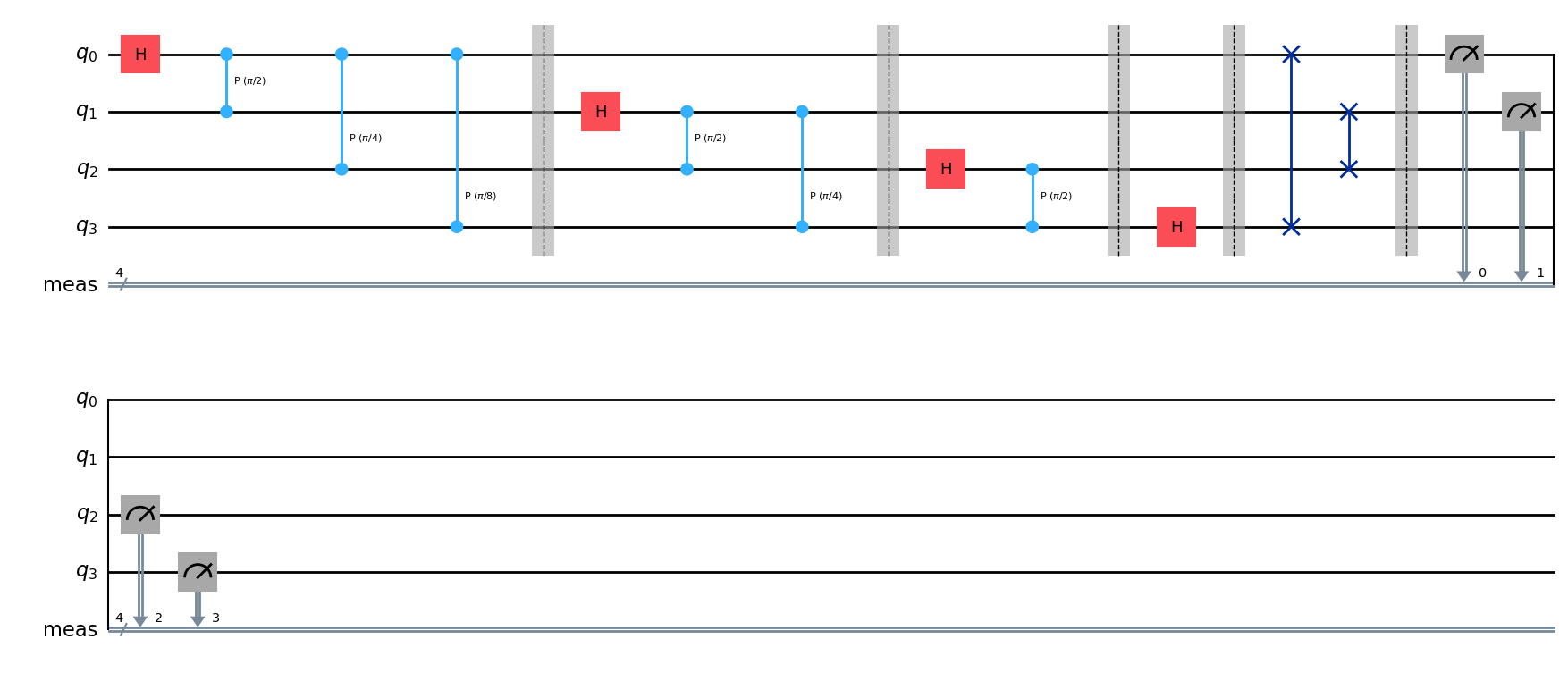
Similarly 2-bit Fourier transformational circuit can be get as follows.
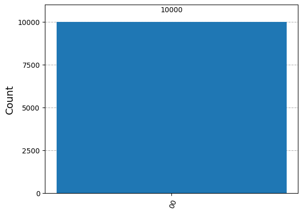
We are going to verify the result in exercise 5.1 that we got earlier.
\(|\psi_1 \rangle =|00\rangle =\begin{pmatrix}1\\0\\0\\0\end{pmatrix}\)
from qiskit import QuantumCircuit import numpy as np def controlled_rotation(qc, control, target, k): """ Adds a controlled rotation gate R_k to the quantum circuit. Parameters: qc (QuantumCircuit): The quantum circuit to which the gate is applied. control (int): The control qubit index. target (int): The target qubit index. k (int): The exponent determining the angle of rotation (2π / 2^k). """ # Calculate the rotation angle (2π divided by 2^k) angle = 2 * np.pi / (2 ** k) # Apply the controlled-phase gate (controlled-R_k) qc.cp(angle, control, target) # Create a 2-qubit quantum circuit (for |00⟩) qcF = QuantumCircuit(2) # No need to initialize; the default state is |00⟩ in Qiskit # Apply a Hadamard gate to qubit 0 to create a superposition qcF.h(0) # Hadamard gate on qubit 0 # Apply controlled rotations with qubit 0 as the target controlled_rotation(qcF, control=1, target=0, k=2) # Controlled R_2 gate qcF.barrier() # Add a barrier to separate different sections of the circuit # Apply a Hadamard gate to qubit 1 qcF.h(1) # Hadamard gate on qubit 1 qcF.barrier() # Barrier after operations on qubit 1 # Swap qubits to reverse the order (commonly done in quantum algorithms like QFT) qcF.swap(0, 1) # Measure all qubits qcF.measure_all() # Print the quantum circuit print(qcF) # Draw the quantum circuit diagram (requires 'matplotlib' to be installed) qcF.draw(output='mpl')Output:
        ┌───┐          ░       ░     ░ ┌─┐
   q_0: ┤ H ├─■────────░───────░──X──░─┤M├───
        └───┘ │P(π/2)  ░ ┌───┐ ░  │  ░ └╥┘┌─┐
   q_1: ──────■────────░─┤ H ├─░──X──░──╫─┤M├
                       ░ └───┘ ░     ░  ║ └╥┘
meas: 2/════════════════════════════════╩══╩═
                                        0  1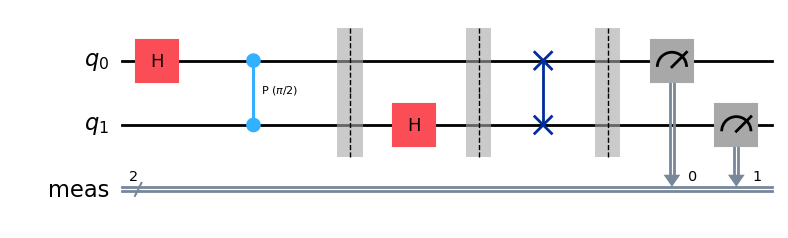
# Importing necessary packages to simulate results

from qiskit import transpile
from qiskit_aer import AerSimulator

backend = AerSimulator()
transpiled_qcF = transpile(qcF, backend)
job = backend.run(transpiled_qcF, shots=10000)    # Shots: Numbers of times the algorithm is run and measured
counts = job.result().get_counts()
print(counts)

from qiskit.visualization import plot_histogram
plot_histogram(counts)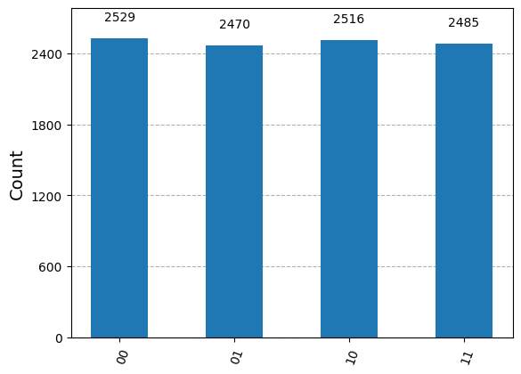
\(|\psi_2 \rangle =|01\rangle =\begin{pmatrix}0\\1\\0\\0\end{pmatrix}\)
from qiskit import QuantumCircuit
import numpy as np

def controlled_rotation(qc, control, target, k):
    """
    Adds a controlled rotation gate R_k to the quantum circuit.

    Parameters:
    qc (QuantumCircuit): The quantum circuit to which the gate is applied.
    control (int): The control qubit index.
    target (int): The target qubit index.
    k (int): The exponent determining the angle of rotation (2π / 2^k).
    """
    # Calculate the rotation angle (2π divided by 2^k)
    angle = 2 * np.pi / (2 ** k)

    # Apply the controlled-phase gate (controlled-R_k)
    qc.cp(angle, control, target)

# Create a 2-qubit quantum circuit
qcF = QuantumCircuit(2)
qcF.initialize([0,1,0,0],[0,1]) #   (for |01>=(1,0,0,0)^T)


# Apply a Hadamard gate to qubit 0 to create a superposition
qcF.h(0)  # Hadamard gate on qubit 0

# Apply controlled rotations with qubit 0 as the target
controlled_rotation(qcF, control=1, target=0, k=2)  # Controlled R_2 gate
qcF.barrier()  # Add a barrier to separate different sections of the circuit

# Apply a Hadamard gate to qubit 1
qcF.h(1)  # Hadamard gate on qubit 1
qcF.barrier()  # Barrier after operations on qubit 1

# Swap qubits to reverse the order (commonly done in quantum algorithms like QFT)
qcF.swap(0, 1)

# Measure all qubits
qcF.measure_all()

# Print the quantum circuit
print(qcF)

# Draw the quantum circuit diagram (requires 'matplotlib' to be installed)
qcF.draw(output='mpl')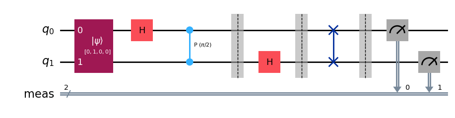
# Importing necessary packages to simulate results

from qiskit import transpile
from qiskit_aer import AerSimulator

backend = AerSimulator()
transpiled_qcF = transpile(qcF, backend)
job = backend.run(transpiled_qcF, shots=10000)    # Shots: Numbers of times the algorithm is run and measured
counts = job.result().get_counts()
print(counts)

from qiskit.visualization import plot_histogram
plot_histogram(counts)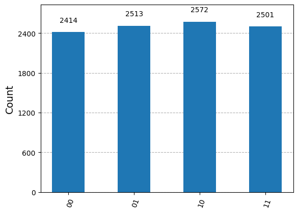
\(|\psi_3 \rangle =\frac{1}{2}\big(|00\rangle+|01\rangle+|10\rangle+|11\rangle\big) =\frac{1}{2}\begin{pmatrix}1\\1\\1\\1\end{pmatrix}\)
from qiskit import QuantumCircuit
import numpy as np

def controlled_rotation(qc, control, target, k):
    """
    Adds a controlled rotation gate R_k to the quantum circuit.

    Parameters:
    qc (QuantumCircuit): The quantum circuit to which the gate is applied.
    control (int): The control qubit index.
    target (int): The target qubit index.
    k (int): The exponent determining the angle of rotation (2π / 2^k).
    """
    # Calculate the rotation angle (2π divided by 2^k)
    angle = 2 * np.pi / (2 ** k)

    # Apply the controlled-phase gate (controlled-R_k)
    qc.cp(angle, control, target)

# Create a 2-qubit quantum circuit
qcF = QuantumCircuit(2)
qcF.initialize([0.5,0.5,0.5,0.5],[0,1]) (for 1/2(|00⟩+|01⟩+|10⟩+|11⟩=1/2(1,1,1,1)^T))


# Apply a Hadamard gate to qubit 0 to create a superposition
qcF.h(0)  # Hadamard gate on qubit 0

# Apply controlled rotations with qubit 0 as the target
controlled_rotation(qcF, control=1, target=0, k=2)  # Controlled R_2 gate
qcF.barrier()  # Add a barrier to separate different sections of the circuit

# Apply a Hadamard gate to qubit 1
qcF.h(1)  # Hadamard gate on qubit 1
qcF.barrier()  # Barrier after operations on qubit 1

# Swap qubits to reverse the order (commonly done in quantum algorithms like QFT)
qcF.swap(0, 1)

# Measure all qubits
qcF.measure_all()

# Print the quantum circuit
print(qcF)

# Draw the quantum circuit diagram (requires 'matplotlib' to be installed)
qcF.draw(output='mpl')
Output
        ┌──────────────────────────────┐┌───┐          ░       ░     ░ ┌─┐
   q_0: ┤0                             ├┤ H ├─■────────░───────░──X──░─┤M├───
        │  Initialize(0.5,0.5,0.5,0.5) │└───┘ │P(π/2)  ░ ┌───┐ ░  │  ░ └╥┘┌─┐
   q_1: ┤1                             ├──────■────────░─┤ H ├─░──X──░──╫─┤M├
        └──────────────────────────────┘               ░ └───┘ ░     ░  ║ └╥┘
meas: 2/════════════════════════════════════════════════════════════════╩══╩═
                                                                        0  1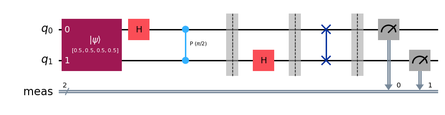
# Importing necessary packages to simulate results

from qiskit import transpile
from qiskit_aer import AerSimulator

backend = AerSimulator()
transpiled_qcF = transpile(qcF, backend)
job = backend.run(transpiled_qcF, shots=10000)    # Shots: Numbers of times the algorithm is run and measured
counts = job.result().get_counts()
print(counts)

from qiskit.visualization import plot_histogram
plot_histogram(counts)